PART1 <求解方程>
1,二分法


def bisect(f,a,b,TOL=0.000004): u_a = a u_b = b while(u_b-u_a)/2.0 > TOL: c = (u_a+u_b)/2.0 if f(c) == 0: break if f(u_a)*f(c) < 0: u_b = c else: u_a = c u_c = (u_a + u_b) / 2.0 return u_cf = lambda x: x*x*x + x - 1ret = bisect(f,-1.0,1.0)print(ret)print(f(ret))
2,不动点迭代法求解方程(FPI)
例如求cosx - x = 0 方程 事实上可以化成x = cosx
x^3 + x - 1 = 0 也可以化成 x=1 - x^3
等式左边是x 右边设为f(x)
即是:x = f(x)
过程如下: x1 = f(x0)x2 = f(x1)x3 = f(x2)........
例如求cosx = x 即(cosx - x = 0)的解: 他的不动点是0.7390851332
def fpi(f,x0,k): xvalues = [] xvalues.append(x0) for i in range(k): xvalues.append(f(xvalues[i])) print(xvalues) return xvalues[-1] # return lastimport mathf = lambda x:math.cos(x)v = fpi(f,0,10)print(v)
上述代码迭代十次 可以看到生成的数值为:
[0, 1.0, 0.5403023058681398, 0.8575532158463933, 0.6542897904977792, 0.7934803587425655, 0.7013687736227566, 0.7639596829006542, 0.7221024250267077, 0.7504177617637605, 0.7314040424225098, 0.7442373549005569, 0.7356047404363473, 0.7414250866101093, 0.7375068905132428, 0.7401473355678757, 0.7383692041223232, 0.739567202212256, 0.7387603198742114, 0.7393038923969057, 0.7389377567153446]
20次基本达到了与精确解
PART2 <求解方程组>
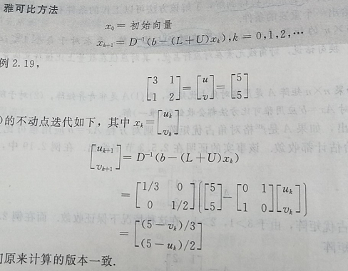
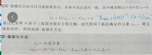
3,雅克比(jacobi)和高斯-赛德尔(Gauss-Seidel) 解方程组
结论:高斯-赛德尔的收敛速度比雅克比快的多。Gauss-Seidel20次迭代达到精确解,jacobi 20次还没得到
还有个高斯-赛德尔SOR 实现起来比较简单。
D代表对角阵,除了对角元素其他都为0
L,除了对角元素往下的元素,其他都为0
U,除了对角元素往上的元素,其他都为0
注意这里的LU和 LU分解是有本质的区别。
高斯赛的尔 用的我蓝色标识的字:
import numpy as npclass GMatrix: @staticmethod def Invert(matrix): nm = np.linalg.inv(matrix.mmatrix) gm = GMatrix() gm.assignNumPyMatrix(nm) return gm def __init__(self, nx=0, ny=0): self.rows = nx self.columns = ny self.mmatrix = np.matrix(np.zeros((nx, ny))) def assignNumPyMatrix(self, matrix): self.mmatrix = matrix def changeShape(self, nx, ny): self.mmatrix = np.matrix(np.zeros((nx, ny))) def debug(self): print("{\n", ">>SHAPE:", (self.mmatrix.shape)) print(self.mmatrix) print('}\n') def numPyMatrix(self): return self.mmatrix def set(self, i, j, var): self.mmatrix[i - 1, j - 1] = var def get(self, i, j): return self.mmatrix[i - 1, j - 1] def L(self): n = self.rows m = GMatrix(n, n) for j in range(1, n, 1): for i in range(j + 1, n + 1): # print(i, j) m.set(i, j, self.get(i, j)) return m def U(self): n = self.rows m = GMatrix(n, n) for i in range(1, n + 1, 1): for j in range(i + 1, n + 1): m.set(i, j, self.get(i, j)) return m def D(self): """ this matrix diagonal values 1,make a empty matrix 2,copy diagonal value to this empty matrix """ n = self.rows m = GMatrix(n, n) for i in range(self.rows): index = i + 1 m.set(index, index, self.get(index, index)) return m def DInvert(self): """ invert diagonal matrix ! :return: """ n = self.rows m = GMatrix(n, n) for i in range(n): index = i + 1 m.set(index, index, 1 / self.get(index, index)) return m def __mul__(self, other): nm = self.mmatrix * other.mmatrix # USE NumPy matrix * matrix m = GMatrix() m.assignNumPyMatrix(nm) return m def __add__(self, other): nm = self.mmatrix + other.mmatrix # USE NumPy matrix + matrix m = GMatrix() m.assignNumPyMatrix(nm) return m def __sub__(self, other): nm = self.mmatrix - other.mmatrix # USE NumPy matrix - matrix m = GMatrix() m.assignNumPyMatrix(nm) return mdef Jacobi_Solver(x0, L, U, invertD, b,iter =20): """ x0 = INIT_VECTOR_VALUE xk+1 = Inv(D)*[ b-(L+U)xk ] ,k = 0,1,2,...... :return: """ nextX = x0 for x in range(iter): nextX = invertD * (b - (L + U) * nextX) return nextXdef Gauss_Seidel_Solver(x0, L, U, D, b,iter =10): """ xk+1 = inv(L+D) * (b- U*xk) """ nextX = x0 for x in range(iter): nextX = GMatrix.Invert(L+D) * (b - U * nextX) return nextXdef unit_test_matrix(): m = GMatrix(2, 2) m.set(1, 1, 3) m.set(1, 2, 1) m.set(2, 1, 1) m.set(2, 2, 2) # and also can this # m.numPyMatrix()[0, 0] = 3 # m.numPyMatrix()[0, 1] = 1 # m.numPyMatrix()[1, 0] = 1 # m.numPyMatrix()[1, 1] = 2 m.debug() m.D().debug() m.L().debug() m.U().debug() m.DInvert().debug()def unit_test_jacobi(): """ | 3 1 | |u| |5| | | | | = | | | 1 2 | |v| |5| -------- AX = b -------- :return: """ # CONSTRUCT THE A MATRIX A = GMatrix(2, 2) A.set(1, 1, 3) # A11 = 3 A.set(1, 2, 1) # A12 = 1 A.set(2, 1, 1) # A21 = 1 A.set(2, 2, 2) # A22 = 2 #A.debug() # CONSTRUCT THE b vector b = GMatrix(2, 1) b.set(1, 1, 5) b.set(2, 1, 5) # INIT zero vector to iter x0 = GMatrix(2,1) # [0,0]T vector initialize invert_D = A.DInvert() L = A.L() U = A.U() print("get the jacobi result ") Jacobi_Solver(x0,L,U,invert_D,b).debug()def unit_test_Gauss_Seidel(): """ | 3 1 | |u| |5| | | | | = | | | 1 2 | |v| |5| -------- AX = b -------- :return: """ # CONSTRUCT THE A MATRIX A = GMatrix(2, 2) A.set(1, 1, 3) # A11 = 3 A.set(1, 2, 1) # A12 = 1 A.set(2, 1, 1) # A21 = 1 A.set(2, 2, 2) # A22 = 2 # CONSTRUCT THE b vector b = GMatrix(2, 1) b.set(1, 1, 5) b.set(2, 1, 5) # INIT zero vector to iter x0 = GMatrix(2, 1) # [0,0]T vector initialize D = A.D() L = A.L() U = A.U() print("get the Gauss_Seidel result ") Gauss_Seidel_Solver(x0, L, U, D, b).debug()unit_test_jacobi()unit_test_Gauss_Seidel()
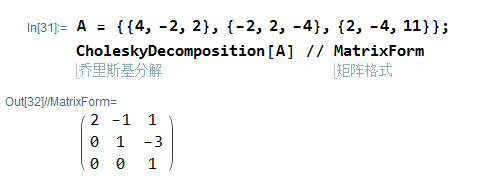
4,楚列斯基分解choleskyDecomposition
这类情况只适合于正定矩阵。
楚列斯基分解的目的就是将正定矩阵分解成A = transpose(R) * R .
求解方程组直接使用回代法即可求出向量解,

这类方法不是迭代法,最重要的是分解矩阵.
所以是要求出来这个上三角矩阵R,比如分解如下矩阵:
[[ 4. -2. 2.] [ -2. 2. -4.] [ 2. -4. 11.]]
import numpy as npimport mathclass GMatrix: def __init__(self, shape): self.nn = shape self.Mat = np.zeros((shape, shape)) def setRawData(self, *args): if len(args) != self.nn * self.nn: raise ValueError deserialize = [] for i in range(self.nn): rhtmp = [] for j in range(self.nn): rhtmp.append(args[i * self.nn + j]) deserialize.append(rhtmp) self.tupleToMatrix(deserialize) def tupleToMatrix(self, tupleObj): """ :param tupleObj: ([1,2],[3,4]) will set matrix above tuple obj """ for i in range(self.nn): # get row data of args row_data = tupleObj[i] for j in range(self.nn): self.Mat[i, j] = row_data[j] def setRowsData(self, *args): if len(args) != self.nn: raise ValueError self.tupleToMatrix(args) def __str__(self): return str(self.Mat) def divideConstant(self, var): self.Mat[:, :] = self.Mat[:, :] / var def __add__(self, other): self.Mat[:, :] = self.Mat[:, :] + other.mat[:, :] def __sub__(self, other): self.Mat[:, :] = self.Mat[:, :] - other.mat[:, :] def nextLayer(self): array = self.Mat[1:, 1:] m = GMatrix(a.Mat.shape[0]) m.Mat = array return m def getupu(self): self.Mat = np.triu(self.Mat) return selfdef choleskyDecomposition(op=GMatrix(2)): """ DEFINE MATRIX: R11 R12 ... R1n R21 R22 ... R2n . . . . . . Rn1 Rn2 ... Rnn """ if len(op.Mat.flatten()) == 1: op.Mat[op.nn - 1:, op.nn - 1:] = np.sqrt(op.Mat[op.nn - 1:, op.nn - 1:]) return # First make the matrix A11 to sqrt(A11) op.Mat[0, 0] = math.sqrt(op.Mat[0, 0]) # R11 op.Mat[0, 1:] = op.Mat[0, 1:] / op.Mat[0,0] # (R12 R13 .... R1n) = (R12 R13 ...R1n) / R11 # cal u.transpose(u) u = np.matrix(op.Mat[0,1:]) # it's a row vector ut = np.transpose(u) # it's a column vector uut = ut*u # extract_layer - uut op.Mat[1:,1:] = op.Mat[1:,1:] - uut choleskyDecomposition(op.nextLayer())a = GMatrix(3)a.setRawData(4, -2, 2, -2, 2, -4, 2, -4, 11)print(a)choleskyDecomposition(a)print(a.getupu())
分解结果R:
[[ 2. -1. 1.] [ 0. 1. -3.] [ 0. 0. 1.]]
Mathematica 检查结果:
5,共轭梯度法:
6,预条件共轭梯度法:
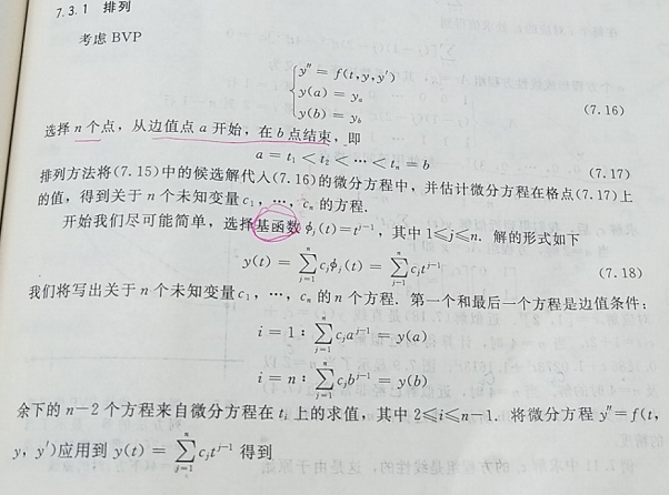
BVP:
差分法比较简单略.
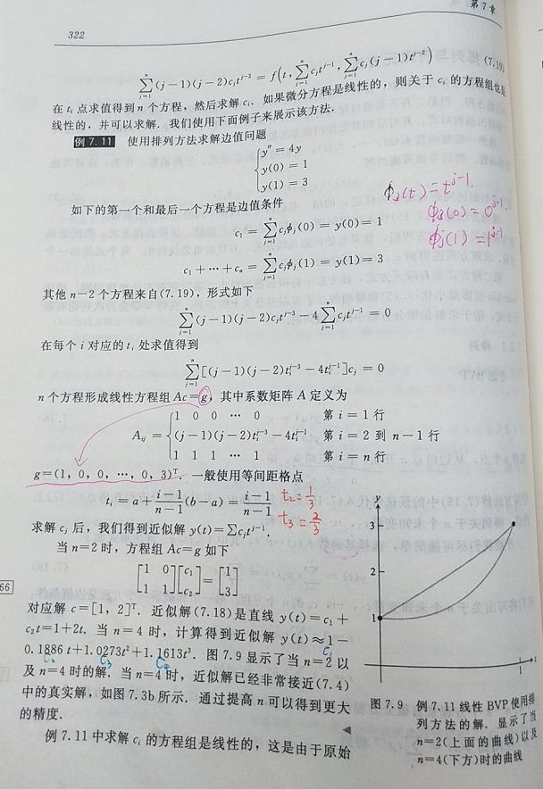
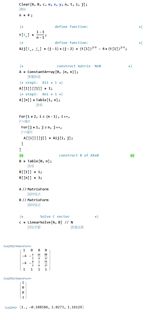
排列法求解BVP问题:
如下例,n=2书中已经给答案,n=4的矩阵未给出,顺便自己解下矩阵n=4的情况。
算出c1,c2,c3,c4:
PDE 解热方程:
这次将时间方向放入坐标轴,可以用三维图像直接看到 在时间步上,热方程是如何传递的.
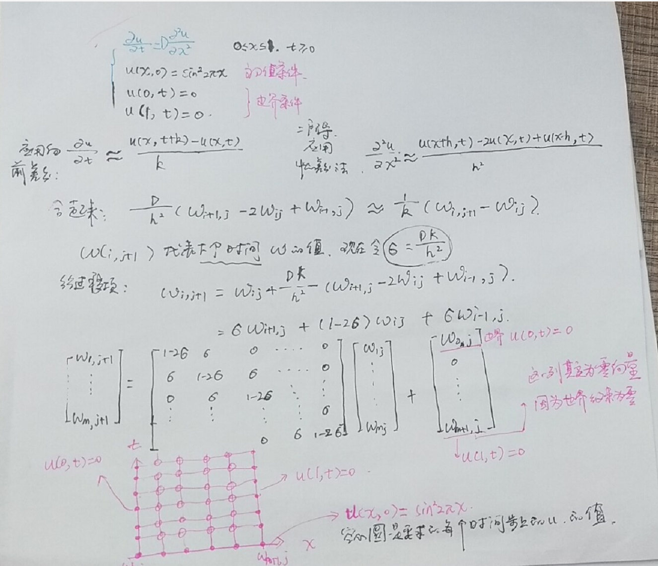
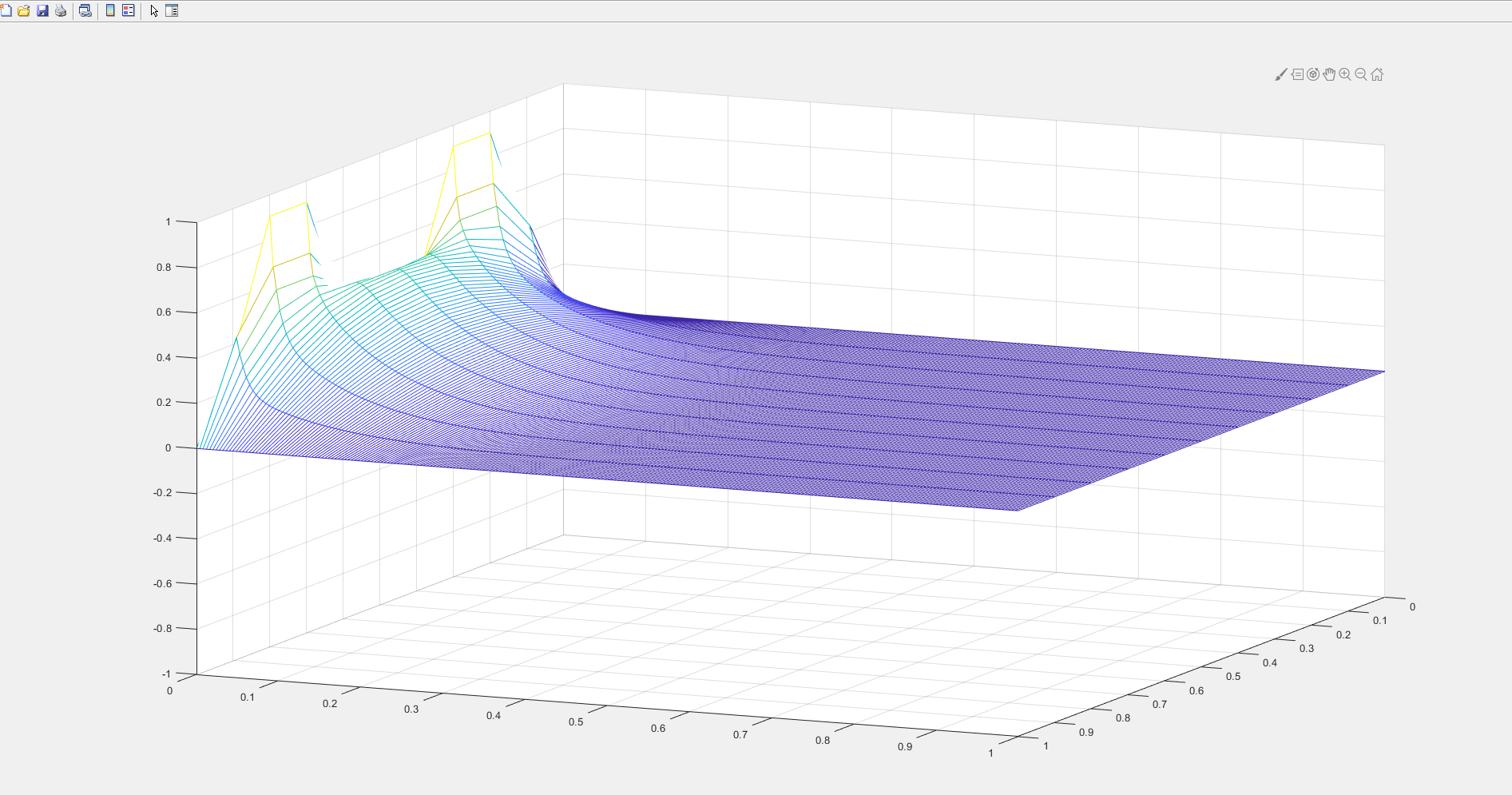
clc;clear w a b c d M N f l r m sigma ;xl = 0;xr = 1;yb = 0;yt = 1;M = 10;N = 250;f = @(x) sin(2*pi*x).^2;l = @(t) 0*t;r = @(t) 0*t;D =1;h = (xr-xl) / Mk = (yt-yb) / Nm = M -1;n=N;sigma = D*k/(h*h);lside = l(yb+(0:n)*k);rside = r(yb+(0:n)*k);% 定义矩阵aa = diag(1-2*sigma*ones(m,1));a = a + diag(sigma*ones(m-1,1),1); %自身加上 往右offset 1列 sigma倍数a = a + diag(sigma*ones(m-1,1),-1); %自身加上 往左偏移 1列sigma倍数a% 设置w第一列 ,初值条件,注意 要转置,因为 设置 w的第一列向量w(:,1) = f(xl + (1:m) * h)'disp('START FOR LOOP')% 给w 在时间250 迭代成列向量,则w是251列向量for j = 1:n rhs = w(:,1)'; w(:,j+1) = a*w(:,j) ;enddisp('END FOR LOOP')w = [lside;w;rside];x = (0:m+1)*h; t= (0:n)*k;mesh(x,t,w')view(60,30);axis([xl xr yb yt -1 1]);